ML Algorithms: Linear Regression

In this post, I discuss what Linear Regression is, the mathematics behind it, and the pros and cons of the algorithm!

supervised learning

To start, let’s have a small refresher on what supervised learning is. Supervised learning is the process of using a dataset ALONG with its associated labels to train a model. There are two major subsets of tasks in supervised learning: 1) classification, and 2) regression. In classification, we aim to separate our data into categories. For example, we could train a model to classify emails as normal or spam using the content of the email. In regression, we aim to predict something in the future. An example of regression would be using current and previous stock prices and other features to determine the stock price in the future. Linear regression is a type of supervised learning algorithm, meaning that our dataset must contain the labels for each data point.

What is linear regression?

Linear regression is a type of supervised learning algorithm that is suitable for regression problems (as the name suggests). The algorithm aims to produce a linear function of the feature set in the form

$y = \theta_0 + \theta_1 x_1 + \theta_2 x_2 + ... + \theta_n x_n + bias$

The theta terms in our equation above are the parameters that the algorithm tweaks during the training phase. The error term accounts for random noise in the data.

Typically, we use $\theta$ to refer to a vector of all of the individual theta terms and X to refer to our feature vector. Therefore, we have $\theta = [\theta_0, \theta_1,...,\theta_n]^T$ and $X = [x_o, x_1,...,x_n]$ . Our model now becomes $y = \theta X + bias$ .

Cost function

In linear regression, we use a cost function to quantify how well our algorithm is performing with our current parameters. The most commonly used cost function is Mean Square Error. For this, we try and minimize the following:

$L(\theta) = \frac{1}{n}\sum_{i=1}^{n} (y_i - x_i \theta)^2$

In words, this cost function tries the minimize the square of the difference between the actual value and the predicted value.

There are other cost functions such as Root Mean Squared Error and Mean Absolute Error. Although I will not be going over these cost functions in this post, a quick google search can help you understand more about these. Each cost function is useful in its own way and can be used based on the situation.

using normal equation

The first method of minimizing the cost function that we are going to look at is using the normal equation.

First, we will take the cost function from above and rewrite it using matrices. We will use $y$ for the labels, $X$ for the feature matrix, and $\theta$ for the parameters we are training.

Now the equation looks like this:

$L(\theta) = \frac{1}{n} (y - X \theta)^T (y - X \theta)$

Now, we can take the partial derivative of $L(\theta)$ in terms of $\theta$ to get $\frac{\partial{L(\theta)}}{\partial{\theta}} = -\frac{2}{n} X^T y + \frac{2}{n} X^T X\theta = 0.$

Solving for $\theta$ , we get $\theta = (X^T X)^-1 X^T y = X^ + y$ where $X^ +$ denotes the pseudo-inverse of $X$ if the inverse cannot directly be calculated.

The disadvantage of this method is that it is computationally expensive.

Gradient descent

In gradient descent, we aim to slowly reduce the cost function in small increments until we reach a local/global minimum. Imagine you have are at the top of a slope and that you are trying to get to the bottom of whatever slope you are at. That is what gradient descent is basically doing. The height of the slope represents how large your cost function value is and we are trying to inch our way down the slope.

The gradient descent algorithm is as follows:

$\theta ^ {t+1} = \theta^t + \frac{\alpha}{n} \sum_{i=1}^{n} x_i ^ T (y_i - x_i \theta)$

The two main factors that influence our gradient descent algorithm are learning rate ( $\alpha$ ) and our starting parameters.

Learning rate

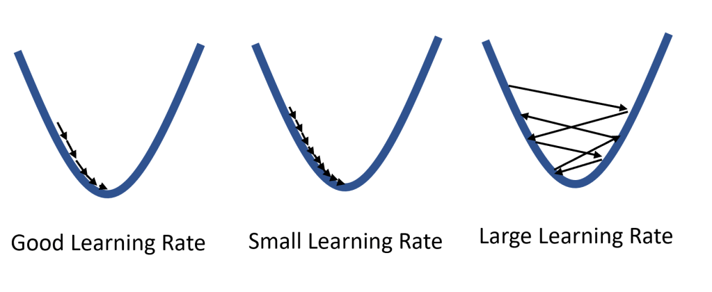
Learning rate, denoted by $\alpha$ , is how fast we are going to be going down the slope. Why does this rate matter? If the learning rate is too large for our dataset, then instead of converging at the minimum value, we will miss the minimum value and go to the other side of the hill. If our learning rate is too small, then the algorithm will take a significantly long time to run

The only way to select a good learning rate is by trial and error. You can try several values and then see which range of values works the best. You can also research online to see if there have been projects similar to your project and see what learning rate worked for their project.

Starting parameters

The starting parameters for our algorithm will play a large role in whether or not we reach the global minimum.

Imagine that instead of just hill, there is a whole mountain range now. Lets say that you are at some peak and that you walked all the way down from the peak to the valley using gradient descent. Are you guaranteed to be at the valley of lowest elevation in the mountain range? No, because there are other valleys in the mountain range that could be at a lower elevation than yours.

This issue occurs when the initialized parameters leads you to a local minimum value instead of the global minimum. To solve this, there are a couple of things you can try.

First, you can try to run your algorithm with new initial parameters until you get better results. This isn’t the most efficient way of solving this problem but it gets the job done.

Another solution is to use an optimizer. For example, the Adam optimizer is commonly used because it gives the algorithm “momentum” as it tries to find the global minimum. This allows it to go over small peaks in hopes of finding the global minimum.

Lastly, you can use a variation of gradient descent called stochastic gradient descent. In stochastic gradient descent, the cost function is evaluated using a different set of data points. This allows the gradient descent algorithm to not get stuck a local minimum value as easily.

Pros and cons

There are pros and cons for each of the algorithms we discussed above.

Pros for Normal Equations:

To solve for theta, there is a single equation that we can use, meaning that this algorithm is the extremely simple to implement

Cons for Normal Equations:

The equation is very computationally expensive
- $latex (X^T X)^{-1} takes a long time to compute
The matrix could be singular

Pros for Gradient Descent:

Converges to a local/global minimum quickly
Easy to implement

Cons for Gradient Descent:

Each iteration of gradient descent requires all of the data to be read

Pros for Stochastic Gradient Descent:

Each iteration is not as computationally expensive as gradient descent because entire dataset is not looked at
Can avoid getting stuck at a local minimum

Cons for Stochastic Gradient Descent:

The values of the cost function will fluctuate frequently
May take a longer time to converge at a value

Summary

Linear regression is one of the most commonly used algorithms in machine learning because it is very easy to understand and easy to implement. Linear regression algorithms have been proven to be highly effective for regression problems.

ML Algorithms: Linear Regression

supervised learning

What is linear regression?

Cost function

using normal equation

Gradient descent

Learning rate

Starting parameters

Pros and cons

Summary

Published by Chaitu Konjeti

Leave a comment Cancel reply

supervised learning

What is linear regression?

Cost function

using normal equation

Gradient descent

Learning rate

Starting parameters

Pros and cons

Summary

Share this:

Related

Published by Chaitu Konjeti

Leave a comment Cancel reply