ML Algorithms: Decision Trees

In today’s post, I will be discussing what Decision Trees are, how they work, and when to use them! This is a high-level introduction to how decision trees work and I hope to provide more in-depth information in future posts.

Introduction

Decision Trees are a commonly used Machine Learning algorithm that most of you have probably encountered before. The algorithm, in essence, splits the data into categories via different attributes until all the data can be classified. The algorithm produces a flowchart-type structure through which all data can be passed through. Don’t worry if that doesn’t make sense just yet. We will delve deeper into the intrinsic mathematics that goes into the development of a Decision Tree.

What is a decision tree?

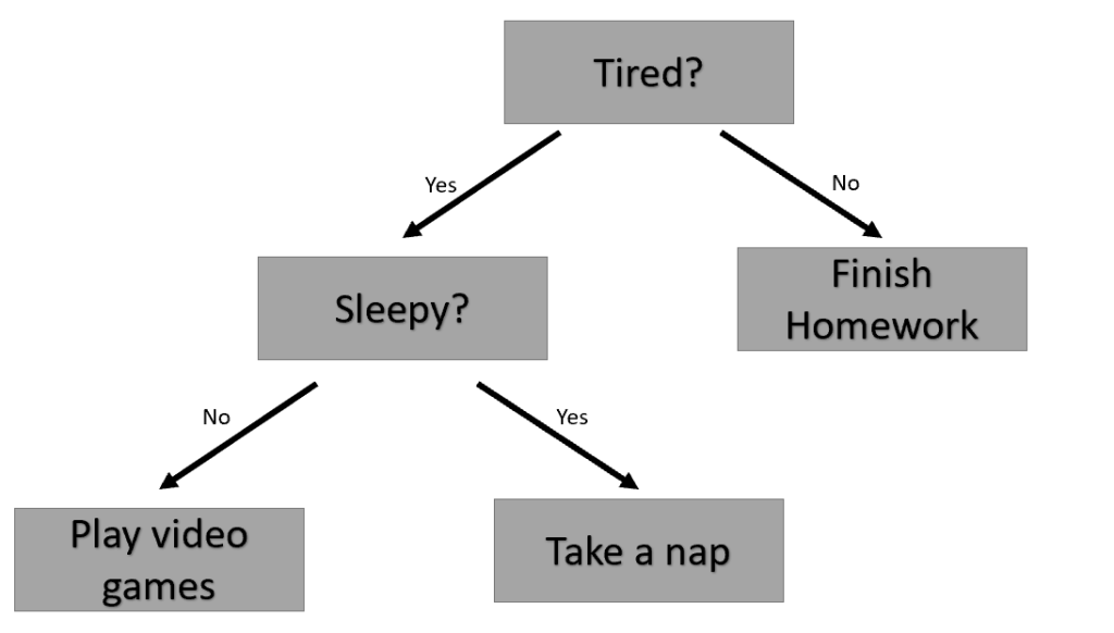
In the example Decision Tree above, we are trying to decide what to do based on how tired and sleepy we are. For example, if we aren’t tired right now, we should finish our homework. However, if we are tired but aren’t sleepy, then we should play some video games to relax. This is essentially what a Decision Tree does. Based on the features of your data, the algorithm creates a tree with branches that split the data into one of two categories until everything can be classified as a leaf node.

how is a decision tree made?

Making a decision tree isn’t a difficult task; however, making the decision tree efficient and as simple as possible requires many more calculations for entropy and information gain (don’t worry, I will discuss what these are in more detail). These calculations help the decision tree minimize the number of branches it has so that the classification occurs as quickly as possible. Let’s take a look at an example.

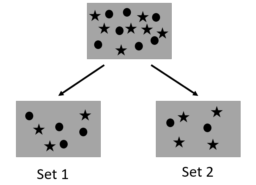
In the picture above, we see that the attribute that we are splitting on causes two smaller groups of data points. In order to make our Decision Tree efficient, we need to make the ideal split. An ideal split would split the data into two groups that are as “pure” as possible, meaning it only contains data from one class label. When you have datasets that contain a lot of attributes and data points, it is not always possible to produce “pure” groups using only one split. However, we will still aim to get our groups as close to one class label as possible.

Entropy

Entropy, in mathematics, refers to the amount of chaos or disorder. In our case, entropy refers to how “unpure” our groups are. In our example above, we want to calculate entropy for each group to see how ideal our split is.

The equation for entropy is the following:

where is the number of the class labels and is the probability of a class label.

So what exactly is this equation saying?

To calculate entropy, you take the classes in your dataset. Then, you calculate what the probability of each class being present in that group is. Lets take a look at our earlier example again and calculate the entropy for each set.

In set 1, the probability of having a circle is and the probability of a star is $\frac{3}{7}. Now, we have all the required variables to compute entropy of set 1.

So now, we need to calculate it for the other set too.

So what information do we have right now? If we use the split attribute that they used in the example, our resulting groups will have the entropy that we calculated above. Our next step is to calculate which split attribute results in the smallest amount of entropy by using information gain.

Information Gain

Information Gain is the measure of how much entropy was reduced by splitting using a particular attribute. The split attribute with the highest information gain will be the one that is used in the final tree.

Information Gain is calculated using the following equation:

where is the entropy of the original group; and are the entropy of the left node and entropy of right node; and and are the probability that a datapoint will go to the left node and the probability that a datapoint will go to the right node.

When to stop splitting

Once a node in the tree only contains data from a single node, we denote the node as a leaf node. Once we have a leaf node, we do not do any further splitting of that node because it is already “pure.” If we have a node that contains data from different classes but can’t be split, then we call this node a leaf node as well. This occurs when data from different classes have the same attributes and cannot be distinguished using the current feature set. We continue branching out until all nodes are leaf nodes.

pros and cons

Decision trees are powerful algorithms for many reasons; however, they do have some drawbacks that you should be aware of. Decision trees perform feature selection when choosing split attributes. They are also capable of working with both numerical and categorical data. This algorithm requires minimal data preparation. Lastly, the decision tree can properly classify data regardless of the type of relationship between parameters. However, there are some drawbacks as well. Decision trees often overfit the data, meaning that it cannot handle data that wasn’t part of the training dataset properly. If there are some classes in the dataset that occur more often than others, the decision tree may show bias towards those classes.

solutions for overfitting

Overfitting occurs for decisions trees when we do not have enough training data and have several unnecessary features. To avoid overfitting, we can add more training data and manually remove features that do not provide important information.

There are also two techniques that can be used to combat overfitting issues: 1) pruning, 2) ensemble learning. I will go into more detail into these techniques in the following sections.

pruning

Pruning is the removal of subtrees that do not provide a lot of useful information for classification. In pruning, we remove the subtree and replace it with a leaf node. We choose to remove a subtree if the subtree produces a larger number of errors than a leaf node would during training and validation.

Ensemble learning

Ensemble learning is when several models are generated and then combined together for final classification and prediction. In the case of decision trees, we can utilize techniques such as Bagging and Random Forest.

Bagging, AKA bootstrap aggregation, is the process of creating smaller subsets of data by taking several random samples from the original dataset with replacement. A decision tree is trained for each subset and then the average of all predictions is used.

Random Forest is an extended version of bagging; for Random Forest, a random set of features is taken along with the subsets of data. In this case, we have a large set of different trees that are being trained on various sets of data. Hence, we have a “random forest” of decision trees. Like bagging, we take the average of the predictions from all trees for our final predictions.

Random Forest is a good ML model to use when you have a large feature set. Random Forest algorithms are also typically good at working with datasets that have missing values. However, the main downside to ensemble learning is that regression models will not be very precise due to the fact that we are aggregating our predictions from many smaller models.